Machine learning is about extracting knowledge from data. When most people think of machine learning or AI, they imagine large companies or academic research teams.
However, it’s relatively straightforward to implement machine learning solutions using Python on your own PC. In this article, we use a popular Python library, scikit-learn, to create four models for predicting the transfer market value of football players. This builds on the simple web scraping used to calculate the best Bundesliga champions.
It’s worth highlighting a key difference here. A transfer fee is the compensation the buying club pays to the selling club if a player transfers before their contract expires. A transfer market value is an estimate of the amount for which a team can sell the player’s contract to another team.
The two values can be markedly different. In 2017, Neymar was sold by Barcelona to PSG for €222 million. At the time, his market value was only just over €100 million.
In this article, we focus on transfer market value.
Setting up
To create a machine learning model, we need data to “learn” from. We’re interested in whether we can use statistical data to predict transfer market values. So, we need data on the transfer market values of certain players, and statistical data for those same players.
KPMG has compiled the Football Benchmark, containing several datasets including market value analytics and sporting performance analytics. In its full version, data is available for more than 8,000 players from top European, South American, and Asian leagues. The free version (requires registration) includes data for 220 of these players, which should be enough to train a relatively reliable model.
I exported the data into Excel, combined each player’s valuation with their performance data, and then masked categorical variables.
Categorical variables are ones described by words rather than numbers. For example, the club a player plays for, or whether they are left- or right-footed. Machine learning models don’t work well with such data, and so they need to be “masked”.
Masking involves turning categorical data into numerical values. To do this, I assigned each categorical variable as follows:
- Club – I assigned each club a bin based on its UEFA coefficient. This meant that the European elite were assigned to bin one, regular Champions League teams to bin two, regular Europa League teams to bin three, and so on.
- League – I assigned each league a mask based on its UEFA coefficient/world ranking, ranging from the Premier League to the Superliga Argentina.
- Position – I assigned each specific position (e.g. attacking midfielder) to a bin based on its overall position on the pitch. Forwards were put in in bin one, midfielders in bin two, and defenders in bin three. Please note, due to their specialised skills, goalkeepers were excluded from this exercise.
- Foot – I assigned each of left-, right-, or two-footed a numerical mask.
- Age – I grouped ages into numbered bins with two-year ranges. Players younger than 20 went into bin one, players between 20 and 22 into bin two, players between 22 and 24 into bin three, and so on.
- Nationality – I assigned each nationality a bin based on FIFA rankings at the time of writing. The top four nationalities were assigned to bin one, the remainder of the top ten to bin two, the remainder of the top 25 to bin three, and all others to bin four.
Once I had satisfactorily masked the data, I imported it to a Pandas DataFrame, ready to begin training the models.
Machine learning problems
There are two major types of machine learning problems, called classification and regression.
In classification, the goal is to predict a class label, which is a choice from a predefined list of possibilities. An example would be training a model to identify whether an email is spam or not.
Regression involves predicting a continuous value from a set of inputs. As this article is interested in predicting transfer market values, we focus on regression models.
Model one – k-nearest neighbours
The first model I use is the k-nearest neighbours model (k-NN). The k-NN algorithm is arguably the simplest machine learning algorithm. To make a prediction for a new data point, the algorithm finds the closest data points (“nearest neighbours”) in the training dataset. The number of nearest neighbours under consideration is a configurable parameter (the k in k-NN).
In any supervised machine learning model, we split the data into a training set and a test set. The training set is the data the model “learns” from. The test set is the data we use to evaluate the model’s predictions.
We use the Root Mean Squared Error (RMSE) to evaluate the model. Because of the way it is calculated, it has the same units as the market value (€m). This allows us to easily understand each model’s performance. A value of zero indicates perfect predictions. The higher the RMSE, the worse the predictions.
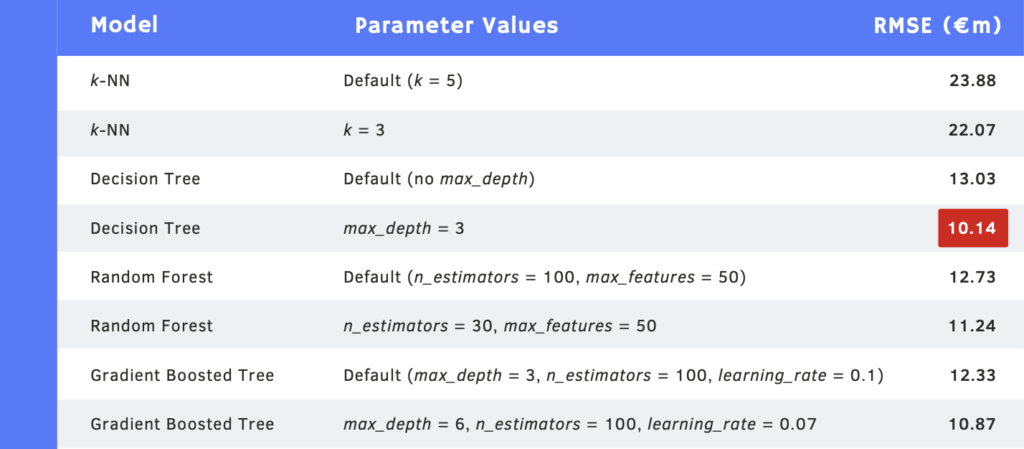
Using the default number of nearest neighbours (5), the model has a RMSE of €23.88m. This means that, for each predicted transfer market value, the true value could be €24 million higher or lower.
Deriving the best parameters
We can adjust k to find the value that gives the lowest RMSE.
Considering each value of k from one to 20 gives the following graph:
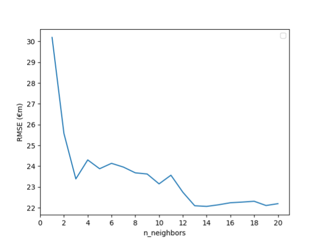
We can see from the graph that the minimum RMSE is €22.07m, which occurs when the number of nearest neighbours is 14.
This is not a huge improvement on the RMSE when k is the default value. The advantage of using k-NN is that it’s conceptually easy to understand. However, it can be slow to predict and does not handle large numbers of features well.
Model two – decision trees
To improve the predictions, the next model I use is a decision tree. This algorithm works by learning a hierarchy of if/else questions, leading to a final result. By default, it continues until each leaf (the terminal node of the tree) is pure, which often leads to overfitting.
This gives an RMSE of €13.03m, which is already much better than the k-NN model.
We can control the overfitting by pre-pruning, which restricts the depth of the tree. This is set via the max_depth parameter.
Deriving the best parameters
We can now adjust max_depth to find the value that gives the lowest RMSE.
Considering each value of max_depth from 1 to 20 gives the following graph:
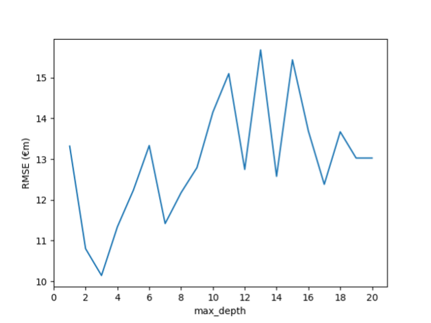
From the graph, we can see that the minimum RMSE is €10.14m, occurring when max_depth is 3. This is a definite improvement on the RMSE with no initial max_depth value. The main drawback of decision trees is that even with the use of pre-pruning, they tend to overfit. Therefore, the ensemble methods we discuss next are usually used in place of a single decision tree.
Model three – random forest
An ensemble combines multiple machine learning models to create an overall more powerful model. One example of a decision tree ensemble is called a random forest.
A random forest is a collection of decision trees, with each tree slightly different to the others. Each individual tree might predict relatively well, but will still overfit on part of the data. If we build many trees, all of which overfit on different parts of the data, we can reduce the amount of overfitting by averaging across their results.
One main parameter is n_estimators, the number of trees in the forest. By default, this is set to 100. The other main parameter is max_features, the number of features each tree looks at for its prediction. For regression tasks, the default is max_features = n_features, where n_features is the number of features in the dataset (in our case, 50).
With these default parameters, the RMSE is €12.73m. Surprisingly, this is actually slightly higher than that from a single decision tree.
Deriving the best parameters
As before, we can adjust n_estimators to find the value that gives the lowest RMSE. The below graph shows the effect of considering each n_estimators (in steps of 10) from 10 to 200.
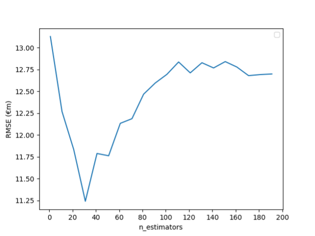
From the graph, we see that the minimum value of RMSE is €11.24m, which occurs when n_estimators is 30. However, this is still outperformed by the single optimised decision tree we saw earlier.
Model four – gradient boosted tree
Another ensemble method made up of multiple decision trees is the gradient boosted tree. Gradient boosting works by building trees in an iterative manner, where each tree tries to correct the mistakes of the previous one.
By default, there is no randomisation in gradient boosted regression trees and pre-pruning is used instead. Gradient boosted trees often use very shallow trees, which makes the model smaller in terms of memory and makes predictions faster.
Apart from the pre-pruning and the number of trees in the ensemble, another important parameter of gradient boosting is the learning_rate, which controls how strongly each tree tries to correct the mistakes of the previous trees. A higher learning_rate means each tree can make stronger corrections, allowing for more complex models.
Using the default values (max_depth = 3, n_estimators = 100, learning rate = 0.1), we get an RMSE of €12.33m. This is slightly better than the default random forest, but still not as good as the single optimised decision tree.
Deriving the best parameters
Altering the max_depth and learning_rate parameters allows us to find the optimum parameters for our problem.
The below 3D graph shows the effect on RMSE of having a max_depth from 1 to 20, and a learning_rate from 0.01 to 0.1.
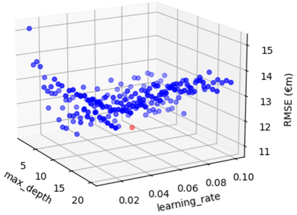
From this graph, we can see that the minimum RMSE (the red point on the graph) is €10.87m, corresponding to a max_depth of 6 and a learning_rate of 0.07. This is closer to the RMSE value from a single optimised decision tree but is still not an improvement.
Conclusion
Despite being prone to overfitting, the optimised single decision tree gave the most accurate predictions, as evidenced by the smallest RMSE of €10.14m.
I trained the models on the free Football Benchmark dataset. This included the 150 most valuable players, plus 70 representatives from the other featured leagues. As such, the data skews towards higher transfer market values. Therefore, the models would likely not generalise well to players with lower market values.
To improve this, I could train the models on a larger dataset with a wider range of transfer market values. Other areas for improvement could include separating each model by position, and including a wider range of metrics, such as those that could indicate popularity (social media mentions, Google searches, merchandise sales etc.).